
Carbon footprint of fuels
All fuels, if you look deeply enough, induce greenhouse gas (GHG) emissions at some point in their life-cycle. I calculate carbon footprints of fossil fuels and biofuels following the international standards organization standard ISO 14067. The full carbon footprint of a fuel includes the emissions associated with extracting the raw materials, transportation, refining, distribution, and combustion.
Coal and oil reserves usually include a certain amount of methane (natural gas) as well, which is a powerful greenhouse gas that can escape to the atmosphere during coal mining or oil drilling. Transportation and distribution of the primary feedstock and the refined fuels burns additional fossil fuels in ships, trucks, and railroad locomotives. Refinery processes requires significant energy, which is supplied by burning some of the feedstock, consuming separate fuel streams, or some of each. For most fossil fuels, the GHG emissions of all these processes add about 20% to the GHG emissions from combusting the final, refined fuel.
I can always calculate combustion emissions for fossil fuels very accurately since they are closely correlated to the mass of the fuel. The transportation, refining, and distribution emissions can also be pretty precise, provided I have access to industrial records of whichever entity is extracting and refining the fuel. Emissions from extracing the feedstock are much more poorly known, and I typically provide estimates of these drawn from published literature. Natural gas suffers from an additional unknown, gas (methane) leakage along pipelines. The extraction emissions are almost always the greatest uncertainty in a carbon footprint of a fuel.
Participating in clean fuels markets
Most of the time that I am conducting life-cycle assessments of fuels, my clients are working toward certification of a carbon intensity value under California’s Low Carbon Fuel Standard (LCFS) program. I specialize in novel “Tier 2” pathways that advance the state of the art in renewable fuels development. My client CleanFuture, Inc., for example, has pioneered the delivery of electricity for transportation from generators located on-site at dairy manure digesters. California LCFS Tier 2 pathways are required to be assessed with the fuel life-cycle assessment tool CA-GREET, which is an adaptation of the GREET model developed at Argonne National Laboratory. So I know this model well, and can help you out with any projects that requires its use.
I have also worked on assessing fuel pathways registered under the Oregon Clean Fuels Program and under British Columbia’s BC-LCFS. Oregon bases fuel pathway assessment on its own adaptation of GREET, OR-GREET, while British Columbia builds from assessments in the Canadian model GHGenius.
In 2021 and 2022, I will be participating in the rulemaking leading to Washington State’s own clean fuels program, as legislated in 2021 House Bill 1091.
Special considerations for biofuels
When calculating carbon footprints of biofuels, I generally follow the U.S. EPA’s proposed Framework for Assessing Biogenic CO2 Emissions from Stationary Sources, making any exceptions needed to remain consistent with my primary standard, ISO 14067. Though the Framework is designed to apply to stationary sources (biomass-fired power plants), most of the concepts and procedures it outlines apply equally well to accounting emissions from liquid biofuels used in mobile sources. The framework calls for calculation of a “biogenic assessment factor” that adjusts the carbon content in the biofuel for net feedstock growth on the production landscape, and several other, secondary factors. Hopefully, the biogenic assessment factor is less than one, meaning that carbon flux at the production landscape offsets some of the emissions from biofuel combustion. But surprisingly often this is not the case, at least when assessing biofuels on a short timescale.
Since growth on the landscape makes all the difference in computing the biogenic assessment factor, I try to model this carefully and thoroughly, usually using the US Forest Service’s Forest Vegetation Simulator. In collaboration with NRDC and the Spatial Informatics Group, I worked on one such analysis to estimate carbon balances of wood pellets manufactured in the U.S. Southeast:
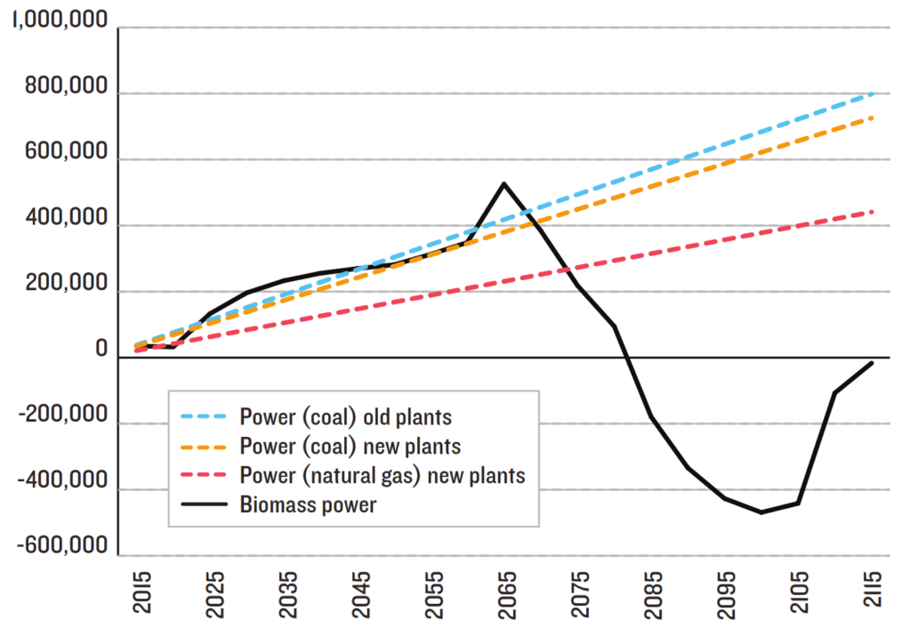
The Y-axis reports cumulative GHG emissions, in metric tons of carbon dioxide equivalent per installed megawatt of wood pellet-fired electric generation. The cumulative emissions from the pellet-based power plant keep pace with the emissions of a conventional coal plant for decades, and finally drop below the cumulative emissions of a modern, natural gas-fired power plant some 60 years after deployment. The main reason for this disappointing outcome, is that by harvesting the landscape the biofuel manufacturer has foregone a high rate of carbon sequestration in a growing, mature forest and replaced it with a much lower rate of carbon sequestration in a new, early forest. It takes about half a century before the new forest can sequester as much carbon as the previous, mature forest would have over the same time period.
But the results from carbon footprint analyses of biofuels are not always so disappointing. Especially fuels that are derived from existing grasslands, for example, can have very encouraging GHG profiles.
Carbon profiles of energy cariers
For most people “fuels” mean combustible materials. Heat or electric energy carriers transmit energy extracted from a fuel, or from another energy resource, to remotely located users. The carbon profiles associated with energy carriers come with some unique issues of their own. Here are energy flows I calculated for a natural gas-fired district heating system, that occasionally co-fires some biomass:
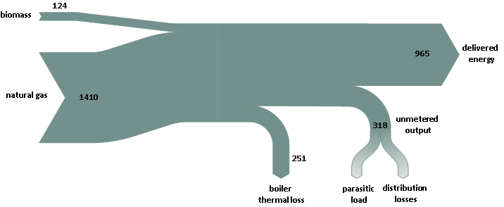
On this particular campus, received heat at the buildings was metered relatively primitively. I calculated unmetered output by subtracting metered, delivered energy from boiler output, which turned out to be about 1/3 the size of the metered, delivered energy. That’s high enough I suspect that some of the unmetered output was in fact delivered to the buildings. But because we had no proof of this we assumed it was lost on the way, either as parasitic load in the power plant (energy consumed by plant equipment), or distribution losses in the hot water and steam pipes. Energy that is “lost” through real distribution loss or through incomplete accounting increases the carbon intensity experienced by the end-users in the buildings, because then the fixed quantity of carbon in the boilder fuel has to be shared among a smaller pool of known use. I have been surprised by how frequently industrial operations and even energy companies operate with very large energy accounting losses like the “unmetered output” in the graphic. If you choose to track and control the GHG intensity of an energy product, you will quickly become aware of how critical accurate metering of fuel and energy flows is.
Utilities, which usually utilize more than a single, owned power plant, face additional uncertainties associated with the vaguaries of the grid. In particular, medium to large utilities all purchase and sell electricity on the spot market, such that the portfolio of generators responsible for the net purchase is unknowable. Some utilities also commit to power purchase agreements that identify only a mix of generating resources, such that the utility cannot know the relative contribution from each, specific plant. When these situations arise I will make assumptions based on the characteristics of the utility’s region and the power plants located there. I can usually do better than the regional averages provided by eGRID, though that tool is always available as a safe backstop.